Analysis of Interferometric Wavefront Data

In this example, we will see how to use prysm to almost entirely supplant the software that comes with a commerical interferometer to analyze the wavefront of an optic. We begin by importing the relevant classes and setting some aesthetics for matplotlib.

from prysm import Interferogram, FringeZernike, sample_files, zernikefit

from matplotlib import pyplot as plt
plt.style.use('bmh')

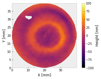
We point prysm to the file, create a new interferogram, mask it to a circular region 100 mm across, subtract piston, tip/tilt and power, and evalute the PV and RMS wavefront error. We also plot the wavefront to make sure all has gone well

p = sample_files('dat')  # sample Zygo .dat file, will be downloaded on demand and saved locally
i = Interferogram.from_zygo_dat(p)
i.crop().mask('circle', 40).crop()
i.remove_piston_tiptilt_power()
print(i.pv, i.rms)
i.plot2d(clim=100, interp_method='bilinear')  # +/- 100 nm
plt.grid(False)

83.33634959318245 15.245987053549815

The interferogram is cropped twice – once to enclose the valid data, then again to apply a mask centered on that region. For relatively conventional interferometry, you may want to stop here. If you want to use a different unit, that is easy enough,

i.change_phase_unit('waves')
1/i.pv, 1/i.rms  # print reciprocal -- "one over xxx waves"

(18.962651752261532, 103.65207382701372)

There is no need to crop again since the outer bound has not changed. Perhaps you wish to evaluated the RMS within the 1 - 10 mm spatial periods,

i.change_phase_unit('nm')
i.fill()
i.bandlimited_rms(1,10)

9.51382202472974

This value is derived from the PSD, so you must call fill first. Do not worry about the corners of the array containing data - it will be windowed out. If you do this on a part which has a central obscuration, the result will be incorrect. Otherwise, the value tends to agree to within +/- 5% of Zygo’s Mx ® software, though the authors of prysm do not believe they are calculated at all the same way.

If you wish to decompose the wavefront into Zernike polynomials, that is easy enough.

# do this on data which has not been filled to avoid errors introduced by the fill value.
coefficients = zernikefit(i.phase, terms=36, norm=True, map_='fringe')
fz = FringeZernike(coefficients, dia=i.diameter, opd_unit=i.phase_unit, norm=True)
fz

rms normalized Fringe Zernike description with:
    -1.195 Z1 - Piston
    -0.271 Z2 - Tilt Y
    +0.484 Z3 - Tilt X
    -2.172 Z4 - Defocus
    -1.351 Z5 - Primary Astigmatism 0°
    +0.324 Z6 - Primary Astigmatism 45°
    -0.217 Z7 - Primary Coma Y
    -1.655 Z8 - Primary Coma X
    -0.241 Z9 - Primary Spherical
    +3.036 Z10 - Primary Trefoil Y
    -1.244 Z11 - Primary Trefoil X
    +1.381 Z12 - Secondary Astigmatism 0°
    -0.049 Z13 - Secondary Astigmatism 45°
    +2.384 Z14 - Secondary Coma Y
    -1.735 Z15 - Secondary Coma X
    +6.297 Z16 - Secondary Spherical
    +1.349 Z17 - Primary Tetrafoil Y
    -0.166 Z18 - Primary Tetrafoil X
    -0.842 Z19 - Secondary Trefoil Y
    +0.229 Z20 - Secondary Trefoil X
    +0.423 Z21 - Tertiary Astigmatism 0°
    -0.040 Z22 - Tertiary Astigmatism 45°
    -1.042 Z23 - Tertiary Coma Y
    +1.362 Z24 - Tertiary Coma X
    -2.779 Z25 - Tertiary Spherical
    +0.171 Z26 - Primary Pentafoil Y
    +0.020 Z27 - Primary Pentafoil X
    -0.235 Z28 - Secondary Tetrafoil Y
    +0.046 Z29 - Secondary Tetrafoil X
    -0.005 Z30 - Tertiary Trefoil Y
    -0.005 Z31 - Tertiary Trefoil X
    -0.489 Z32 - Quaternary Astigmatism 0°
    +0.025 Z33 - Quaternary Astigmatism 45°
    +0.106 Z34 - Quaternary Coma Y
    -0.192 Z35 - Quaternary Coma X
    +0.307 Z36 - Quaternary Spherical
    45.208 PV, 9.334 RMS [nm]

This print might be a bit daunting, one may prefer to see the top few terms by magnitude,

fz.top_n(5)

[(6.296543, 16, 'Secondary Spherical'),
 (3.035946, 10, 'Primary Trefoil Y'),
 (-2.779492, 25, 'Tertiary Spherical'),
 (2.38442, 14, 'Secondary Coma Y'),
 (-2.171752, 4, 'Defocus')]

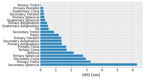
or a barplot of all terms,

fz.barplot_magnitudes(orientation='v', sort=True)

(<Figure size 432x288 with 1 Axes>,
 <matplotlib.axes._subplots.AxesSubplot at 0x7f1ca453a7f0>)

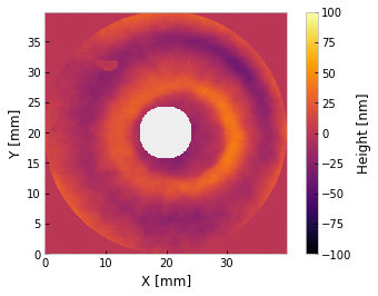
The sample data has a ciruclar clear aperture, but if it had a central obscuration (such as transmitted wavefront data for a telescope) that would be easy to mask too. PSD, and by extension bandlimited RMS values for data with annular support will be nonsensical.

i.mask('invertedcircle', 7)
i.plot2d(clim=100)  # +/- 100 nm
plt.grid(False)